Vania Esady and Stephen Burgess
A summary measure for UK households’ resilience
High levels of household debt have been shown to amplify recessions. For example, in the global financial crisis (GFC), UK households with more debt tended to cut back their spending disproportionately, amplifying aggregate demand effects and potentially making the recession worse. High levels of household (and corporate) debt can pose risks to the UK financial system through two main channels: lender resilience and borrower resilience. However, monitoring households’ resilience to future shocks is not an easy task. In this post we construct some new summary measures of borrower resilience. We show that increases in debt-servicing costs or in the flow of credit to households could make households less resilient overall.
Our contribution
How resilient are households to shocks? To answer this require knowing today, how much households might cut their spending by, if they were stressed in the future. We show a way to do this, and we link our measure to key aggregate measures of household debt.
Our approach draws on previous research by Aikman et al (2019) and Adrian et al (2019), who model the whole distribution of GDP growth, conditional on several financial variables such as debt levels and asset prices. These approaches are now used in policy institutions like the Federal Reserve Bank of New York for regular risk monitoring. More recently, Schmitz (2022) shows how monetary policy can influence a monthly index of downside risks to consumption growth. However, as far as we know, we are the first authors to apply these approaches to UK household spending.
What we do
We work with annual growth in UK household consumption, and use an approach known as quantile regression – a statistical tool that allows us to estimate the relationship between a range of risk indicators and the whole distribution of possible consumption outcomes. In a standard regression model, a relationship is fitted to minimise the squared errors between consumption growth and some explanatory factors, but quantile regression focuses on particular points in the distribution – say the 5th or 10th percentile – and minimises a weighted sum of positive and negative error terms. Repeating this exercise for different quantiles shows the broad overall shape of the distribution of consumption growth.
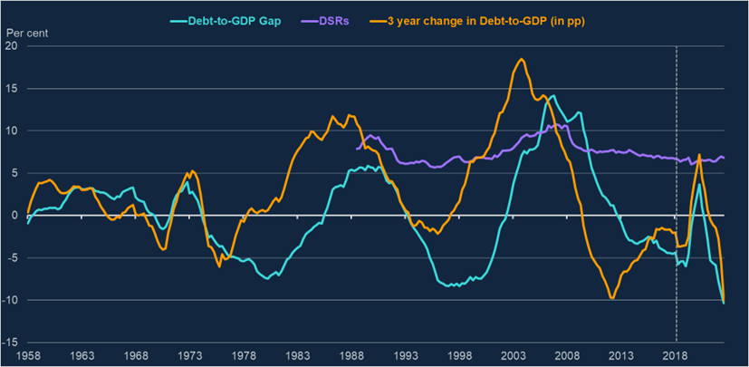
How do we choose our explanatory factors? We draw on a combination of previous research and on risk indicators that the Financial Policy Committee regularly monitor, and we compare potential models using a Continuous Ranked Probability Score approach. Roughly speaking, this ranks models depending on how good their density forecasts are, when considered out-of-sample. All of our models use lagged annual consumption growth and the change in the unemployment rate over three years as explanatory factors. We also include in the regression three different measures of household vulnerabilities (Chart 1): the household sector debt-service ratio (DSR); a measure of the household debt-to-GDP ‘gap’ (similar to the BIS measure for total private sector debt); and household credit growth, defined as the change in household debt as a share of GDP over three years. In this post we use these in three separate model specifications. The data are available since 1980, except for the DSR which begins in 1989. We estimate the models up to 2019 (vertical dashed line in Chart 1) to avoid the distortions in the data caused by Covid. This means the model is missing Covid and other support measures for the economy after 2019 that could have impacted spending decision.
Chart 1: Household debt metrics
Sources: Bank of England, ONS and authors’ calculations.
What we find
The panels in Chart 2 show how our risk indicators influence tail risks to household spending growth. We interpret our results as helpful relationships present in recent UK data, rather than claiming they provide evidence of a causal link. The solid blue lines plot the quantile regression coefficients from our in-sample estimates and the shaded areas show confidence intervals. Within each panel, the lines show the effect at different quantiles of the distribution. Reading across, the three columns show results from the three different models. Reading down, the charts show the effect of the debt measures on consumption growth at one and three-year horizons respectively. If the solid blue line is significantly below zero, it means the debt measure is expected to pull down on spending growth at that horizon. If it is sloping, it means debt affects the shape of the distribution as well as the average. For example, in the top-left panel, DSRs influence spending growth by more at the left tail than they do at the median.
We highlight these results from Chart 2:
- In year one, high DSRs have a significant negative impact on the left tail of consumption growth, and by more than at the median.
- Comparing across the three different models, the DSR coefficients are also numerically the biggest. A one standard deviation increase in household DSRs lowers consumption growth at the 5th percentile by 1.4 percentage points (top-left panel).
- When we estimate additional models with two or three debt variables, the DSR variable tends to explain more of the variation than the other two (not shown in the chart).
- The results for the debt gap show it having a negative effect on consumption growth, but less of an effect on the shape of the distribution.
- For credit growth, the most significant effects are at the three-year horizon (bottom-right panel), and the coefficients are more significant at the left tail than at the median.
Chart 2: Estimated quantile regression coefficients from our models
Notes: Solid blue lines denote median coefficient estimates, light (dark) blue-shaded areas represent 90% (68%) confidence bands from block bootstrap procedure. Models include macroeconomic controls: three-year unemployment change and lagged quarterly consumption growth (annualised).
Source: Authors’ calculations.
We can look at these through a different lens by focusing on the 5th percentile and plotting the coefficients through time (Chart 3). For the DSR measure, the effect on consumption growth peaks at the three-quarter horizon and then diminishes, consistent with other work that finds the medium-term effect of DSRs to be smaller. On the other hand, the impact of credit growth on spending takes five quarters to build up, but then remains significant.
Chart 3: Quantile regression coefficients through time, for the 5th percentile
Note: Solid blue lines denote median coefficient estimates, light (dark) blue-shaded areas represent 90% (68%) confidence bands from block bootstrap procedure.
Source: Authors’ calculations.
Finally, we can measure how risks to spending have changed over time, from early 1990s to 2023. We use the in-sample estimated coefficients in Chart 2 to calculate the risk measures in Chart 4. We argue that summary measures like this could be helpful to policymakers. For simplicity, we focus just on our model using DSRs.
The blue line (shortfall) shows the 5th percentile of the future distribution of spending, and we invert it so that a higher value implies higher risk. For example, the 5th percentile is consistent with no spending growth at the one-year horizon, but growth of around 1.5% at the three-year horizon. That reflects the fact that the DSRs have been rising a little recently (Chart 1), but DSRs matter much more for spending in the near term than further out.
A complementary way to measure household resilience is to look at the ‘Downside risks’. While the blue line considers a certain point (5th percentile) of the distribution, the orange line takes the entire probability mass below the median into account. In more technical terms, to describe downside risks, we can use relative entropy: the excess probability mass above or below a certain quantile, in this case below the median, of the conditional distribution relative to the probability mass of the unconditional density. The blue line in Chart 4 shows that during recessionary periods, we could expect relatively more probability mass in the left side of the conditional distribution, which raises downside risks.
Chart 4: Two measures of downside risks to spending conditional on DSRs
Note: For more details of the methodology, we would refer interested readers to Section II.B in Adrian et al (2019).
Source: Authors’ calculations.
Implications
Chart 4 shows that there has not been excessive household debt growth over the past 15 years. Household risk measure has remained contained ever since the aftermath of the GFC (ignoring volatility associated with Covid). Over the past two years, households have not carried out drastic spending cuts, despite facing rising living costs and rising interest rates, because they entered this period in a more resilient position.
What would happen if household borrowing growth were to pick up in the future? The right-hand panel of Chart 3 shows it could take 1–2 years for the maximum effect on consumption to come through, providing time for any macroprudential policies to be implemented. By contrast, if policy action was only taken when higher credit flows had fed through to a notably higher level of debt or of DSRs, borrower resilience would already be at the point of deteriorating (the first and second panels in Chart 3).
Vania Esady works in the Bank’s Current Economic Conditions Division. This post was written while Stephen Burgess was working in the Bank’s Macrofinancial Risks Division.
If you want to get in touch, please email us at [email protected] or leave a comment below.
Comments will only appear once approved by a moderator, and are only published where a full name is supplied. Bank Underground is a blog for Bank of England staff to share views that challenge – or support – prevailing policy orthodoxies. The views expressed here are those of the authors, and are not necessarily those of the Bank of England, or its policy committees.
Share the post “A summary measure for UK households’ resilience”
Publisher: Source link


